Big Picture
Tutorials 4-6 tested individual aspects of randomness: aggregate frequencies (chi-squared), single probabilities (Beta-Binomial), and all 69 balls independently (Dirichlet-Multinomial). Each test passed. The lottery appears fair.
But these tests make a critical assumption: independence. They assume Ball 23's probability is unaffected by Ball 41. They assume the machine does not change over time. They assume patterns do not exist across sequences of draws.
This tutorial explores what happens when we try to test relationships, temporal patterns, and conditional dependencies. You will discover why the combinatorial explosion of possibilities makes manual analysis impossible, and why automated pattern search (neural networks) becomes necessary.
1. Where We Are in the Journey
Tutorial 1-3 built clean data and features. Tutorial 4-6 tested whether individual balls follow random distributions. All tests passed. We have strong evidence that no single ball is biased.
But "no individual ball is biased" is not the same as "the lottery is random." There could be patterns we have not tested yet. Maybe Ball 23 and Ball 41 appear together too often. Maybe the machine changed in 2020. Maybe patterns exist across time.
This tutorial asks: can we test ALL possible patterns? The answer will lead us to neural networks.
2. Eliminating Simple Explanations
Before diving into complex patterns, we need to rule out two simple possibilities: temporal dependence and machine drift.
We test: Are consecutive draws independent? Or do high draws follow high draws (clustering)?
We test: Did the machine change between 2015 and 2024? Or have ball frequencies stayed stable?
These are quick tests (30-40 lines of code each). If they pass, we can focus on the harder problem: ball relationships.
3. The Ball Pair Problem: Conditional Probability
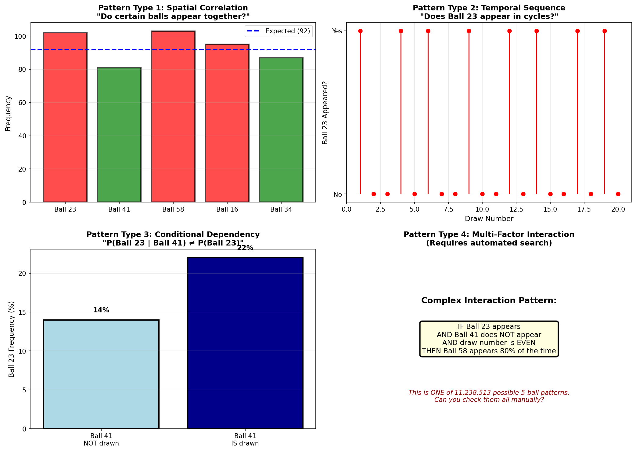
Tutorial 6 tested whether Ball 23 appears too often. It does (102 times vs expected 92). But we declared it "not suspicious" because the credible interval barely excludes the expected value, and we expect 3-4 false positives with 69 balls.
But what if Ball 23 only appears when Ball 41 also appears? That would suggest a dependency: P(Ball 23 | Ball 41) ≠ P(Ball 23). This is a question about conditional probability.
To test this, we build a co-occurrence matrix: how many times each pair of balls appeared together in the same draw.
This is already at the limit of human analysis. A heatmap with 4,761 cells is barely readable. But pairs are just the beginning.
4. The Combinatorial Explosion
We just analyzed pairs. But the lottery draws 5 balls simultaneously. What about triplets? Quadruplets? All 5-ball combinations?

If we could check 1 million combinations per second, testing all 5-ball patterns would take 11 seconds. That sounds manageable. But we also have time.
We have 1,269 draws. Each combination could appear at any point in time. That is 11,238,513 × 1,269 = 14,261,669,097 possible patterns.
And we have not even considered:
- Order of appearance within a draw
- Sequences across multiple draws (Ball A in draw N, Ball B in draw N+1)
- Interactions with the Powerball number
- Machine/vendor effects
- Seasonal patterns, day-of-week effects
5. Why Manual Models Fail
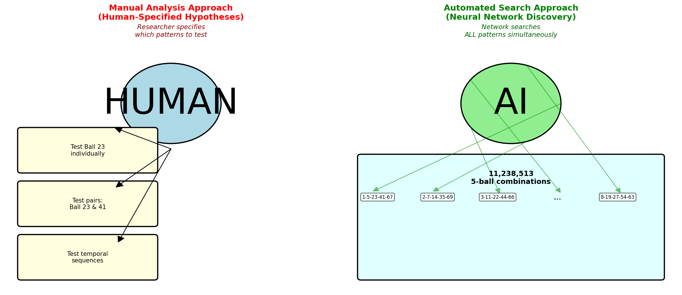
The limitation of every model we have built so far (chi-squared, Beta-Binomial, Dirichlet-Multinomial, runs test, changepoint detection) is that they require us to SPECIFY the pattern we are testing.
Bayesian models are excellent for testing specified hypotheses with proper uncertainty quantification. They are not designed for exploratory search across millions of patterns.
6. Code Walkthrough: Testing the Limits
The script performs four main analyses:
Tests whether consecutive draws are independent or show clustering/oscillation patterns.
Compares ball frequencies in early vs late draws to detect distribution shifts.
Builds a 69×69 matrix showing which ball pairs appear together more/less than expected.
Calculates how many patterns exist and why manual testing is infeasible.
7. Python Implementation
The script is split into 4 parts for clarity. Here is the complete implementation:
"""Tutorial 7: The Dimensionality Crisis - When Manual Analysis Becomes Impossible"""

import pandas as pd
import numpy as np
from scipy import stats
import matplotlib.pyplot as plt
import seaborn as sns
from itertools import combinations

# --- Load cleaned data ---

print("Tutorial 7: The Dimensionality Crisis")
print("=" * 60)
print("\nLoading cleaned Powerball data from Tutorial 1...")
draws = pd.read_parquet('data/processed/powerball_clean.parquet')
print(f"Loaded {len(draws)} draws\n")

# --- PART 1: Eliminate Simple Explanations ---

print("\n" + "=" * 60)
print("PART 1: Eliminating Simple Explanations")
print("=" * 60)

# --- Test 1: Runs Test (Temporal Independence) ---

print("\n[Test 1: Runs Test - Are draws independent over time?]\n")

# Extract mean values from each draw
draw_means = []
for _, row in draws.iterrows():
    balls = [row['ball1'], row['ball2'], row['ball3'], row['ball4'], row['ball5']]
    draw_means.append(np.mean(balls))

draw_means = np.array(draw_means)
overall_median = np.median(draw_means)

# Count runs (sequences above/below median)
above_median = draw_means > overall_median
n_runs = 1
for i in range(1, len(above_median)):
    if above_median[i] != above_median[i-1]:
        n_runs += 1

n_above = np.sum(above_median)
n_below = len(above_median) - n_above

# Expected runs under independence
expected_runs = ((2 * n_above * n_below) / (n_above + n_below)) + 1
variance_runs = (2 * n_above * n_below * (2 * n_above * n_below - n_above - n_below)) / \
                ((n_above + n_below)**2 * (n_above + n_below - 1))
std_runs = np.sqrt(variance_runs)

# Z-test
z_score = (n_runs - expected_runs) / std_runs
p_value = 2 * (1 - stats.norm.cdf(abs(z_score)))

print(f"  Observed runs: {n_runs}")
print(f"  Expected runs (if independent): {expected_runs:.2f}")
print(f"  Z-score: {z_score:.4f}")
print(f"  P-value: {p_value:.4f}")

if p_value >= 0.05:
    print(f"  ✓ PASS: Draws appear independent over time (p >= 0.05)")
else:
print(f" ✗ FAIL: Evidence of temporal dependence (p < 0.05)")# --- Test 2: Changepoint Detection (Temporal Stability) ---
print("\n[Test 2: Changepoint Detection - Did the machine change?]\n")
# Split data into two halves and compare ball frequency distributions
midpoint = len(draws) // 2
early_draws = draws.iloc[:midpoint]
late_draws = draws.iloc[midpoint:]
# Count ball frequencies in each period
def count_ball_frequencies(draw_data):
counts = np.zeros(69)
for _, row in draw_data.iterrows():
for ball in [row['ball1'], row['ball2'], row['ball3'], row['ball4'], row['ball5']]:
counts[ball - 1] += 1
return counts
early_counts = count_ball_frequencies(early_draws)
late_counts = count_ball_frequencies(late_draws)
# Chi-squared test for distribution change
chi2_stat, p_value_change = stats.chisquare(late_counts, early_counts)
print(f" Early period: draws 1-{midpoint}")
print(f" Late period: draws {midpoint+1}-{len(draws)}")
print(f" Chi-squared statistic: {chi2_stat:.4f}")
print(f" P-value: {p_value_change:.4f}")
if p_value_change >= 0.05:
print(f" ✓ PASS: No evidence of machine change (p >= 0.05)")
else:
print(f" ✗ FAIL: Ball frequencies shifted between periods (p < 0.05)")
print("\n" + "-" * 60)
print("Conclusion: The lottery is stable and independent.")
print("The problem isn't time or drift. It's something else...")
print("-" * 60)# --- PART 2: The Ball Pair Problem ---
print("\n\n" + "=" * 60)
print("PART 2: The Ball Pair Problem - Conditional Probabilities")
print("=" * 60)
print("\nWe've proven individual balls are fair.")
print("But what if certain balls appear TOGETHER more often than they should?")
# Build co-occurrence matrix
print("\n[Computing all pairwise co-occurrences...]\n")
cooccurrence_matrix = np.zeros((69, 69))
for _, row in draws.iterrows():
balls = [row['ball1'], row['ball2'], row['ball3'], row['ball4'], row['ball5']]
# For each pair of balls in this draw
for i, ball_a in enumerate(balls):
for ball_b in balls[i+1:]:
cooccurrence_matrix[ball_a - 1, ball_b - 1] += 1
cooccurrence_matrix[ball_b - 1, ball_a - 1] += 1 # Symmetric
# Compute expected co-occurrences and correlations
ball_frequencies = np.zeros(69)
for _, row in draws.iterrows():
for ball in [row['ball1'], row['ball2'], row['ball3'], row['ball4'], row['ball5']]:
ball_frequencies[ball - 1] += 1
expected_cooccurrence = np.outer(ball_frequencies, ball_frequencies) / (len(draws) * 5)
expected_cooccurrence = expected_cooccurrence * 4
correlation_matrix = cooccurrence_matrix - expected_cooccurrence
print(f" Matrix size: 69 × 69 = {69*69} cells")
print(f" Unique pairs: {69*68//2} combinations")
# Save correlation heatmap
plt.figure(figsize=(14, 12))
sns.heatmap(correlation_matrix, cmap='RdBu_r', center=0,
xticklabels=range(1, 70), yticklabels=range(1, 70),
cbar_kws={'label': 'Deviation from Expected Co-occurrence'})
plt.title('Ball Pair Correlation Matrix\n(69×69 = 4,761 relationships)',
fontsize=14, fontweight='bold')
plt.tight_layout()
plt.savefig('outputs/tutorial7/correlation_matrix.png', dpi=150)
plt.close()
print("\n Saved: correlation_matrix.png")# --- PART 3: The Combinatorial Explosion ---
print("\n\n" + "=" * 60)
print("PART 3: The Combinatorial Explosion")
print("=" * 60)
from math import comb
pairs = comb(69, 2)
triplets = comb(69, 3)
quadruplets = comb(69, 4)
quintuplets = comb(69, 5)
print(f"\n Pairs (2 balls): {pairs:,}")
print(f" Triplets (3 balls): {triplets:,}")
print(f" Quadruplets (4 balls): {quadruplets:,}")
print(f" Quintuplets (5 balls): {quintuplets:,}")
print(f"\n Total 5-ball combinations: {quintuplets:,}")
print(f" If we check 1 million combinations per second:")
print(f" Time required: {quintuplets / 1_000_000:.1f} seconds")
print("\n But we also have TIME.")
print(f" We have {len(draws)} draws.")
print(f" That's {quintuplets:,} × {len(draws)} = {quintuplets * len(draws):,} patterns.")
print("\n" + "-" * 60)
print("The dimensionality is IMPOSSIBLE for manual analysis.")
print("-" * 60)
print("\n" + "=" * 60)
print("THE SOLUTION: Automated High-Dimensional Search")
print("=" * 60)
print("\nThis is why neural networks exist.")
print("\nNeural networks solve a DIFFERENT problem:")
print(" - Bayesian models: Test specified hypotheses")
print(" - Neural networks: Search high-dimensional spaces")
print("\nTutorial 8 will build networks to search this space.")
print("If they find nothing, the lottery is provably random.")
print("If they find patterns, we have evidence of bias.\n")8. How to Run the Script
- You must have run Tutorial 1 first (to create
powerball_clean.parquet) - Create the output folder:
mkdir outputs/tutorial7# Windows (PowerShell)
cd C:\path\to\tutorials
python tutorial7_dimensionality_crisis.py# Mac / Linux (Terminal)
cd /path/to/tutorials
python3 tutorial7_dimensionality_crisis.py9. The Bridge to Neural Networks
We have now exhausted manual analysis. Runs test: PASS. Changepoint test: PASS. Individual balls: PASS. Pairwise correlations: at human limit.
But we cannot test all 11 million 5-ball combinations. We cannot check temporal sequences. We cannot explore conditional dependencies automatically.
Neural networks solve this problem. They do not replace Bayesian models. They serve a different purpose:
A neural network trained on lottery data will try to predict future draws based on past draws. If it succeeds (accuracy significantly above random baseline), we have evidence of patterns. If it fails (accuracy = 1/69 ≈ 1.4%), we have strong evidence the lottery is truly random.
10. What You Now Understand (and the path forward)
You understand the difference between testing individual hypotheses and searching high-dimensional spaces. You know why the combinatorial explosion makes manual analysis infeasible. You see why classical statistical methods (Bayesian or frequentist) cannot scale to millions of pattern combinations.
More importantly, you understand the intellectual progression that leads to neural networks. It is not "old methods bad, new methods good." It is "manual specification works for simple problems, automated search required for complex problems."
We have identified three distinct types of patterns that could exist in lottery data:
Tutorials 8-10 will systematically test each pattern type using the appropriate neural architecture:
Each architecture is designed to solve a specific problem. MLPs process spatial features. LSTMs add temporal memory. Transformers add relational attention. By testing all three systematically, we ensure comprehensive coverage of the pattern space.
Tutorial 8 begins with the simplest case: can a neural network learn to predict draws using only the static features we engineered in Tutorial 2?