Big Picture
Tutorial 4 asked a yes-or-no question: "Is this lottery random?" The chi-squared test gave you a p-value. If p < 0.05, you rejected randomness. If p ≥ 0.05, you failed to reject. But that binary decision discards information. It does not tell you how confident you should be.
This tutorial introduces Bayesian inference. Instead of asking "reject or fail to reject," Bayesian methods ask "what do I believe, and how certain am I?" The answer is not a single number. It is a probability distribution that captures your entire state of knowledge.
You will learn to start with a prior belief, observe data, and compute a posterior belief. As you see more data, the posterior narrows. Your uncertainty decreases. This framework is the foundation of modern machine learning and uncertainty quantification.
1. Where We Are in the Journey
Tutorial 1 filtered the data. Tutorial 2 built features. Tutorial 3 validated distributions. Tutorial 4 ran frequentist hypothesis tests. All of those steps were preparation for statistical inference.
Tutorial 5 is the first module that treats probability as a measure of belief rather than long-run frequency. This is a conceptual shift. In frequentist statistics, a coin has a fixed probability of heads (say, 0.5), and we test whether data is consistent with that fixed value. In Bayesian statistics, the probability itself is uncertain. We have a belief about what it might be, and we update that belief as we observe data.
The workflow: raw data → validated data → feature table → EDA → frequentist tests → Bayesian inference → deep learning.
We are at step six.
2. The Bayesian Mindset: From Tests to Beliefs
In frequentist statistics, you test a null hypothesis. You either reject it or you do not. The decision is binary. The uncertainty is hidden behind a p-value threshold.
In Bayesian statistics, you do not test hypotheses. You update beliefs. You start with a prior distribution that represents what you believe before seeing any data. You observe data. You compute a posterior distribution that represents what you believe after seeing the data.
The key insight: uncertainty is not something to eliminate. It is something to quantify. A Bayesian posterior tells you not just what you believe, but how confident you should be.
3. The Beta Distribution: Encoding Prior Beliefs
Before you see any lottery data, what do you believe about the probability that a draw has 2 or 3 odd numbers? If the lottery is fair, that probability should be around 0.648 (from the binomial distribution). But you are not certain. Maybe it is 0.64, maybe 0.65, maybe 0.60.
The Beta distribution lets you encode that uncertainty. It is a probability distribution over probabilities. It takes two parameters, α and β, that control its shape.
Compare these reference examples showing different prior beliefs:
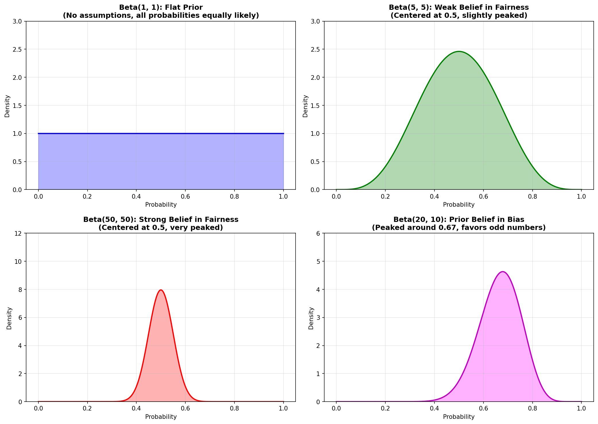
For lottery analysis, we usually start with Beta(1, 1) because we do not want to bias the result with strong prior assumptions.
4. The Update Rule: Prior + Data = Posterior
The beauty of the Beta-Binomial model is that the math is simple. If your prior is Beta(α, β) and you observe k successes in n trials, your posterior is Beta(α + k, β + n - k). That is it. No complex integrals. Just add the observed counts to your prior parameters.
Here is the update rule:
Data: k successes in n trials
Posterior: Beta(α + k, β + n - k)
Every success increments α. Every failure increments β. The posterior encodes all the information from your prior belief and the observed data.
5. Concrete Example: Testing Odd/Even Balance
Let's test whether the lottery is fair by looking at odd/even balance. From Tutorial 2, we know each draw has an odd_count feature. If the lottery is random, we expect about 64.8% of draws to have 2 or 3 odd numbers. This comes from the binomial distribution with n=5 and p=0.5 (from Tutorial 4): P(k=2) + P(k=3) ≈ 0.318 + 0.330 = 0.648.
Prior: Beta(1, 1)
This represents complete ignorance. All probabilities are equally likely.
Out of 1,269 draws, 823 have 2 or 3 odd numbers.
Observed proportion: 823 / 1,269 ≈ 0.6485
Posterior: Beta(1 + 823, 1 + 446) = Beta(824, 447)
The distribution is now very narrow, centered around 0.648.
95% credible interval: [0.623, 0.674]
We are 95% confident the true probability is in this range.
Compare your results to this reference showing how the posterior evolves:
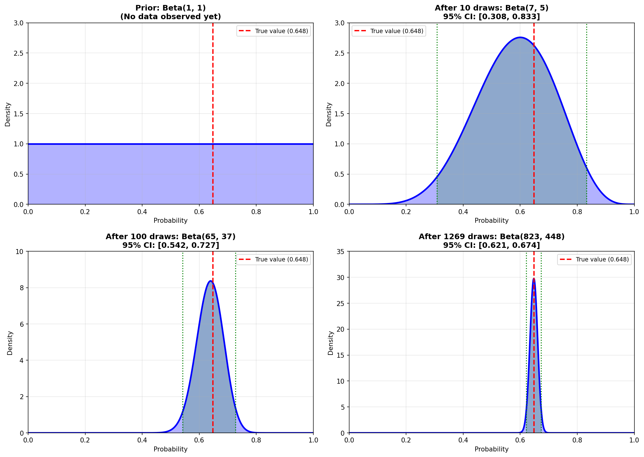
Notice how the posterior starts flat (prior belief) and narrows as we see more draws. After 1,269 draws, we are very confident about the true probability.
6. Code Roadmap: What the Script Does (and Why This Order)
The script performs five main steps:
Read the feature table from Tutorial 2 and count how many draws have 2 or 3 odd numbers.
Start with Beta(1, 1), a flat prior that represents no initial assumptions.
Apply the Beta-Binomial conjugate update: Posterior = Beta(α + successes, β + failures).
Calculate the mean, mode, standard deviation, and 95% credible interval of the posterior.
Plot both distributions to see how beliefs changed after observing data.
7. Python Implementation
Here is the complete script. It performs Bayesian inference on the odd/even balance feature.
"""Tutorial 5: Use Bayesian inference to quantify beliefs about lottery fairness"""

import pandas as pd
import numpy as np
from scipy import stats
import matplotlib.pyplot as plt

# --- Load feature table ---

print("Loading feature table from Tutorial 2...")
features = pd.read_parquet('data/processed/features_powerball.parquet')
print(f"Loaded {len(features)} draws\n")

# --- Extract odd count data ---

odd_counts = features['odd_count'].values
n_draws = len(odd_counts)

# Count how many draws had exactly 2 or 3 odd numbers (close to expected 2.5)
successes = np.sum((odd_counts == 2) | (odd_counts == 3))
trials = n_draws

print(f"Observed data:")
print(f"  Total draws: {trials}")
print(f"  Draws with 2 or 3 odd numbers: {successes}")
print(f"  Proportion: {successes / trials:.4f}")
print(f"  Expected if random: ~0.648 (64.8%)\n")

# --- Define prior ---

# Start with a uniform prior: Beta(1, 1)
# This represents "no prior knowledge"
alpha_prior = 1
beta_prior = 1

print(f"Prior: Beta({alpha_prior}, {beta_prior})")
print(f"  This is a flat prior (all probabilities equally likely)\n")

# --- Bayesian update ---

# The Beta-Binomial conjugate update:
# Posterior = Beta(alpha_prior + successes, beta_prior + failures)
alpha_posterior = alpha_prior + successes
beta_posterior = beta_prior + (trials - successes)

print(f"Posterior: Beta({alpha_posterior}, {beta_posterior})")
print(f"  Updated belief after observing {trials} draws\n")

# --- Compute posterior statistics ---

posterior_mean = alpha_posterior / (alpha_posterior + beta_posterior)
posterior_mode = (alpha_posterior - 1) / (alpha_posterior + beta_posterior - 2)
posterior_std = np.sqrt(
    (alpha_posterior * beta_posterior) /
    ((alpha_posterior + beta_posterior)**2 * (alpha_posterior + beta_posterior + 1))
)

print(f"Posterior statistics:")
print(f"  Mean: {posterior_mean:.4f}")
print(f"  Mode (most likely value): {posterior_mode:.4f}")
print(f"  Std Dev: {posterior_std:.4f}\n")

# --- Compute credible interval ---

# 95% credible interval
# ppf = Percent Point Function (inverse CDF)
# ppf(0.025) gives the value where 2.5% of probability mass is below
# ppf(0.975) gives the value where 97.5% of probability mass is below
lower = stats.beta.ppf(0.025, alpha_posterior, beta_posterior)
upper = stats.beta.ppf(0.975, alpha_posterior, beta_posterior)

print(f"95% Credible Interval: [{lower:.4f}, {upper:.4f}]")
print(f"  We are 95% confident the true probability is in this range\n")

# --- Visualize prior vs posterior ---

print("Creating visualization...")

x = np.linspace(0, 1, 1000)
prior_pdf = stats.beta.pdf(x, alpha_prior, beta_prior)
posterior_pdf = stats.beta.pdf(x, alpha_posterior, beta_posterior)

plt.figure(figsize=(12, 6))

# Plot prior
plt.plot(x, prior_pdf, 'b--', linewidth=2, label='Prior: Beta(1,1)', alpha=0.7)

# Plot posterior
plt.plot(x, posterior_pdf, 'r-', linewidth=2, label=f'Posterior: Beta({alpha_posterior},{beta_posterior})')

# Mark the credible interval
plt.axvline(lower, color='green', linestyle=':', linewidth=1.5, label=f'95% CI: [{lower:.3f}, {upper:.3f}]')
plt.axvline(upper, color='green', linestyle=':', linewidth=1.5)
plt.fill_between(x, 0, posterior_pdf, where=(x >= lower) & (x <= upper),
                 alpha=0.2, color='green', label='95% Credible Region')

# Mark the expected value
plt.axvline(0.648, color='orange', linestyle='--', linewidth=2, label='Expected if random (0.648)')

plt.xlabel('Probability of 2 or 3 Odd Numbers', fontsize=12)
plt.ylabel('Probability Density', fontsize=12)
plt.title('Bayesian Update: Prior to Posterior', fontsize=14)
plt.legend(fontsize=10)
plt.grid(alpha=0.3)
plt.tight_layout()
plt.savefig('outputs/tutorial5/bayesian_update.png', dpi=150)
plt.close()

print("  Saved: bayesian_update.png\n")

# --- Summary ---

print("Summary")
print("-" * 40)
print(f"We started with a flat prior (no assumptions).")
print(f"After observing {trials} draws, our belief narrowed to:")
print(f"  Most likely value: {posterior_mode:.4f}")
print(f"  95% confident range: [{lower:.4f}, {upper:.4f}]")
print(f"\nThe expected value (0.648) falls within our credible interval.")
print(f"Conclusion: The data is consistent with randomness.\n")
8. How to Run the Script
- You must have run Tutorial 2 first (to create
features_powerball.parquet) - Create the output folder:
mkdir outputs/tutorial5# Windows (PowerShell)
cd C:\path\to\tutorials
python tutorial5_bayesian_inference.py# Mac / Linux (Terminal)
cd /path/to/tutorials
python3 tutorial5_bayesian_inference.py9. Interpreting the Posterior
The posterior distribution tells you everything you have learned from the data. Here is how to read it:
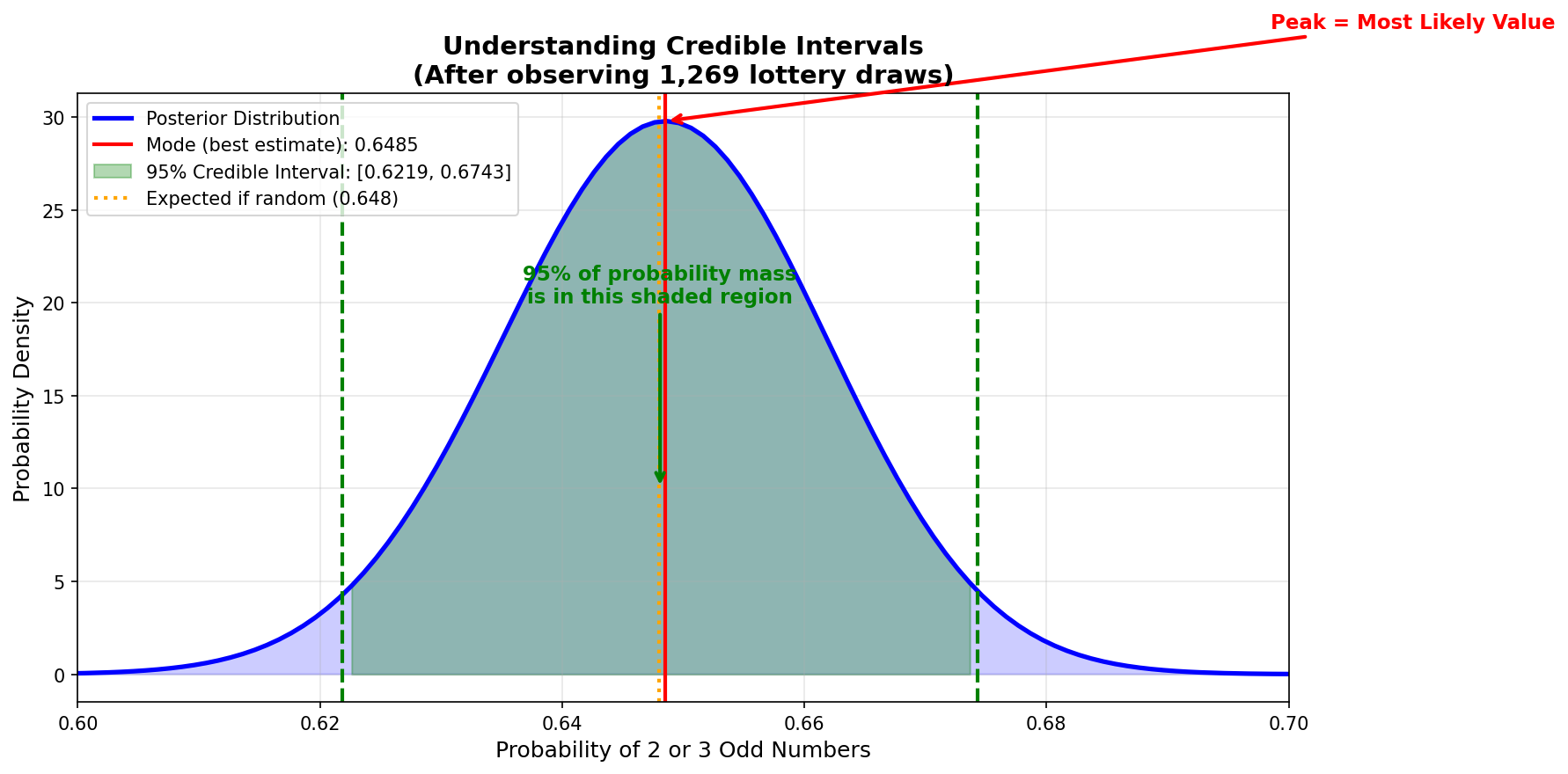
This is your best estimate. For our example, mode ≈ 0.6485. If you had to pick a single number, this is it.
This is your uncertainty. A narrow posterior means high confidence. A wide posterior means low confidence. For our example, std ≈ 0.0134 (very narrow).
This is the range where the true value likely falls. A 95% credible interval means: "there is a 95% probability the true value is in this range." For our example: [0.622, 0.674].
10. What You Now Understand (and why it matters later)
You know how to encode prior beliefs with the Beta distribution. You know how to update beliefs using the Beta-Binomial conjugate model. You can compute posterior statistics and credible intervals. You understand that Bayesian inference quantifies uncertainty rather than making binary decisions.
This tutorial focused on a simple case: testing a single probability (odd/even balance). Tutorial 6 will scale this approach to all 69 balls simultaneously using the Dirichlet distribution. That generalization is the foundation for detecting which specific balls, if any, deviate from randomness.
More importantly, you now understand the Bayesian mindset. Uncertainty is not something to hide behind p-values. It is something to model explicitly. This philosophy carries forward to deep learning, where neural networks output probability distributions rather than point predictions.