Big Picture
Tutorial 5 tested a single probability: "What fraction of draws have 2 or 3 odd numbers?" That question reduces the lottery to a binary outcome (success or failure). But the real lottery has 69 white balls. Each ball has its own probability of being drawn.
This tutorial scales Bayesian inference to handle all 69 balls simultaneously. You will learn the Dirichlet distribution, which is the natural generalization of the Beta distribution from 2 outcomes to K outcomes. You will test whether specific balls are drawn more or less often than they should be.
The key challenge: distinguishing between truly biased balls and balls that just look suspicious because we have not seen enough data yet. The Dirichlet posterior gives you credible intervals for each ball. Wide intervals mean "we need more data." Narrow intervals that exclude the expected value mean "this ball might actually be biased."
1. Where We Are in the Journey
Tutorial 4 used chi-squared tests to check if aggregate features match random expectations. Tutorial 5 introduced Bayesian inference for a single probability. Both approaches treated the lottery as a simplified system.
Tutorial 6 applies Bayesian inference to the full lottery. Instead of reducing 69 balls to a single feature (odd count, mean, etc.), we test all 69 balls directly. This is the first tutorial that treats each ball as an independent question: "Is ball #42 biased?"
The workflow: raw data → validated data → feature table → EDA → frequentist tests → Beta-Binomial inference → Dirichlet-Multinomial inference → deep learning.
We are at step seven.
2. The Challenge: From 2 Outcomes to 69 Outcomes
In Tutorial 5, we had two outcomes: a draw either has 2-3 odd numbers (success) or it does not (failure). The Beta distribution handled that easily. It is a curve over the interval [0, 1] representing the probability of success.
But the lottery has 69 possible outcomes for each pick. The probability space is 69-dimensional. You cannot visualize a 69-dimensional curve. You cannot easily compute marginal probabilities. The math gets harder.
The solution: the Dirichlet distribution. It is the natural generalization of the Beta distribution. Where Beta handles 2 outcomes, Dirichlet handles K outcomes.
3. The Dirichlet Distribution: The Big Brother of Beta
The Dirichlet distribution is a probability distribution over probability vectors. It takes K parameters, α₁, α₂, ..., αₖ, one for each outcome. The distribution is written as Dir(α₁, α₂, ..., αₖ).
Compare these conceptual examples:
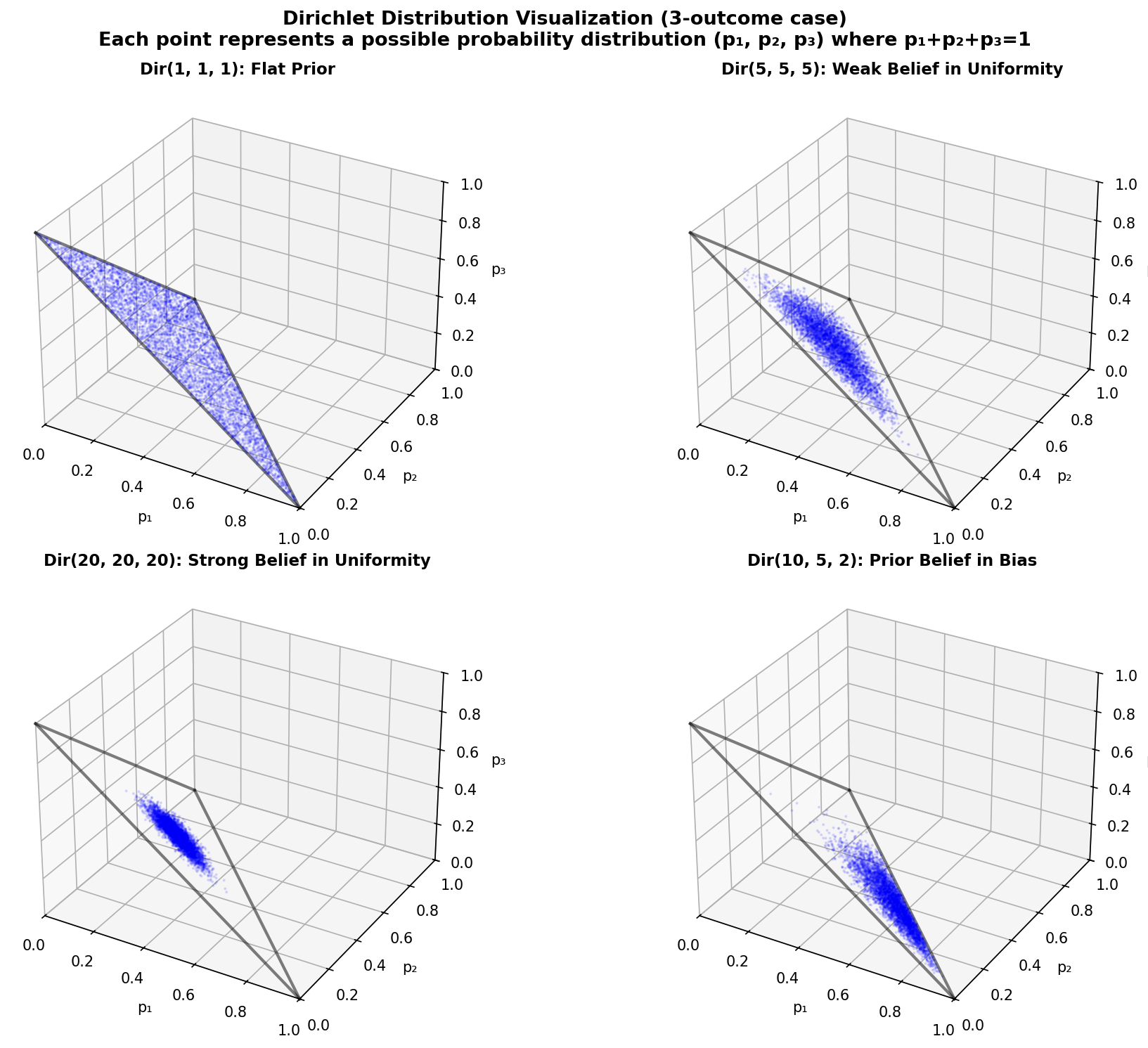
For lottery analysis, we start with Dir(1, 1, ..., 1) to avoid imposing prior assumptions.
4. The Update Rule: Prior + Counts = Posterior
The Dirichlet-Multinomial update is just as simple as the Beta-Binomial update. If your prior is Dir(α₁, ..., αₖ) and you observe counts (c₁, ..., cₖ), your posterior is Dir(α₁ + c₁, ..., αₖ + cₖ).
Here is the update rule:
Data: ball 1 appeared c₁ times, ball 2 appeared c₂ times, ...
Posterior: Dir(α₁ + c₁, α₂ + c₂, ..., α₆₉ + c₆₉)
After 1,269 draws (6,345 total ball picks), each count cᵢ is around 92. The posterior parameters are around 93. The distribution is very narrow. We are confident about the probability of each ball.
5. Concrete Example: Testing All 69 Balls
We will count how many times each ball (1-69) appeared in the 1,269 draws. If the lottery is fair, each ball should appear about 92 times (6,345 total picks / 69 balls ≈ 91.96). We will compute credible intervals for each ball and identify which ones, if any, deviate significantly.
Go through all 1,269 draws. Count how many times each ball appeared.
Example: Ball 7 appeared 95 times, Ball 42 appeared 89 times.
Prior: Dir(1, 1, 1, ..., 1) (69 ones)
This represents no prior belief about which balls are more likely.
Posterior: Dir(1 + c₁, 1 + c₂, ..., 1 + c₆₉)
Example: If ball 7 appeared 95 times, its posterior parameter is 96.
For each ball, compute the 95% credible interval for its probability.
Check if the expected uniform probability (1/69 ≈ 0.01449) falls within the interval.
A ball is "suspicious" if its credible interval does not contain 1/69.
With 69 balls and 95% intervals, we expect about 3-4 false positives even if all balls are fair.
6. Code Roadmap: What the Script Does (and Why This Order)
The script performs six main steps:
Read the cleaned draws from Tutorial 1. Extract all white balls into a single array.
Count how many times each ball (1-69) appeared across all draws.
Start with Dir(1, 1, ..., 1), a flat prior over all 69 balls.
Add observed counts to prior parameters: Posterior = Dir(α + counts).
Use normal approximation to compute 95% credible intervals for each ball's probability.
Create a 7x10 grid showing posterior probabilities for all 69 balls. Mark suspicious balls in red.
7. Python Implementation
Here is the complete script. It tests all 69 balls for deviations from uniformity.
"""Tutorial 6: Use Dirichlet inference to test if specific balls deviate from uniformity"""

import pandas as pd
import numpy as np
from scipy import stats
import matplotlib.pyplot as plt

# --- Load cleaned data ---

print("Loading cleaned Powerball data from Tutorial 1...")
draws = pd.read_parquet('data/processed/powerball_clean.parquet')
print(f"Loaded {len(draws)} draws\n")

# --- Extract ball frequencies ---

# Collect all white balls from all draws
all_balls = []
for _, row in draws.iterrows():
    all_balls.extend([row['ball1'], row['ball2'], row['ball3'], row['ball4'], row['ball5']])

all_balls = np.array(all_balls)
n_total_picks = len(all_balls)  # Should be 5 * n_draws

print(f"Total ball picks: {n_total_picks}")
print(f"  (5 balls per draw × {len(draws)} draws)\n")

# Count frequency of each ball (1-69)
ball_counts = np.zeros(69)
for ball_num in range(1, 70):
    ball_counts[ball_num - 1] = np.sum(all_balls == ball_num)

# Expected frequency if uniform
expected_frequency = n_total_picks / 69

print(f"Expected frequency per ball (if uniform): {expected_frequency:.2f}")
print(f"\nObserved frequencies (first 10 balls):")
for i in range(10):
    print(f"  Ball {i+1}: {ball_counts[i]:.0f} (expected: {expected_frequency:.2f})")
print("  ...\n")

# --- Define prior ---

# Uniform Dirichlet prior: all alpha = 1
# This is the 69-dimensional generalization of Beta(1,1)
alpha_prior = np.ones(69)

print(f"Prior: Dirichlet(α₁=1, α₂=1, ..., α₆₉=1)")
print(f"  This is a flat prior over all 69 balls")
print(f"  Sum of alphas: {np.sum(alpha_prior):.0f} (weak prior, easy to update)\n")

# --- Bayesian update ---

# The Dirichlet-Multinomial conjugate update:
# Posterior = Dirichlet(alpha_prior + counts)
alpha_posterior = alpha_prior + ball_counts

print(f"Posterior: Dirichlet(α₁={alpha_posterior[0]:.0f}, α₂={alpha_posterior[1]:.0f}, ..., α₆₉={alpha_posterior[68]:.0f})")
print(f"  Updated belief after observing {len(draws)} draws")
print(f"  Sum of alphas: {np.sum(alpha_posterior):.0f} (strong posterior, hard to change)\n")

# --- Compute posterior statistics for each ball ---

# Posterior mean for each ball
posterior_means = alpha_posterior / np.sum(alpha_posterior)

# Expected probability if uniform
expected_prob = 1.0 / 69

# Compute credible intervals for each ball
# For Dirichlet, we use the fact that each marginal is approximately normal for large counts
# This is justified by the Central Limit Theorem
lower_bounds = []
upper_bounds = []

for i in range(69):
    # Use normal approximation for the marginal
    # Mean: alpha_i / sum(alpha)
    # Variance: (alpha_i * (sum(alpha) - alpha_i)) / (sum(alpha)^2 * (sum(alpha) + 1))
    alpha_sum = np.sum(alpha_posterior)
    mean = alpha_posterior[i] / alpha_sum
    variance = (alpha_posterior[i] * (alpha_sum - alpha_posterior[i])) / (alpha_sum**2 * (alpha_sum + 1))
    std = np.sqrt(variance)

    # 95% credible interval using ±1.96 standard deviations
    lower = mean - 1.96 * std
    upper = mean + 1.96 * std

    lower_bounds.append(lower)
    upper_bounds.append(upper)

lower_bounds = np.array(lower_bounds)
upper_bounds = np.array(upper_bounds)

# --- Identify suspicious balls ---

# A ball is "suspicious" if the expected uniform probability (1/69)
# falls outside its 95% credible interval
suspicious_balls = []

for i in range(69):
    if expected_prob < lower_bounds[i] or expected_prob > upper_bounds[i]:
        suspicious_balls.append(i + 1)  # Ball numbers are 1-indexed

print(f"Suspicious balls (expected value outside 95% CI):")
if len(suspicious_balls) == 0:
    print("  None! All balls are consistent with uniformity.")
else:
    print(f"  Found {len(suspicious_balls)} suspicious balls:")
    for ball_num in suspicious_balls[:10]:  # Show first 10
        idx = ball_num - 1
        print(f"    Ball {ball_num}: observed {ball_counts[idx]:.0f}, "
              f"expected {expected_frequency:.2f}, "
              f"95% CI: [{lower_bounds[idx]*n_total_picks:.1f}, {upper_bounds[idx]*n_total_picks:.1f}]")
    if len(suspicious_balls) > 10:
        print(f"    ... and {len(suspicious_balls) - 10} more")

print()

# --- Visualize posterior as heatmap ---

print("Creating heatmap visualization...")

# Reshape ball numbers into a 7x10 grid for visualization
# (69 balls don't fit perfectly, so last row will have 9 balls)
grid_data = np.zeros((7, 10))
grid_data[:] = np.nan  # Initialize with NaN

ball_idx = 0
for row in range(7):
    for col in range(10):
        if ball_idx < 69:
            grid_data[row, col] = posterior_means[ball_idx]
            ball_idx += 1

# Create heatmap
fig, ax = plt.subplots(figsize=(14, 8))

# Plot heatmap
# vmin=0.013 and vmax=0.016 are chosen to "zoom in" around the expected value of 1/69 ≈ 0.01449
# This makes small deviations from uniformity more visually apparent in the color scale
im = ax.imshow(grid_data, cmap='RdYlGn_r', aspect='auto', vmin=0.013, vmax=0.016)

# Add colorbar
cbar = plt.colorbar(im, ax=ax)
cbar.set_label('Posterior Probability', fontsize=12)

# Mark expected uniform probability
expected_line = ax.axhline(y=-0.5, color='blue', linestyle='--', linewidth=2, alpha=0)  # Invisible line for legend
ax.plot([], [], color='blue', linestyle='--', linewidth=2, label=f'Expected (1/69 = {expected_prob:.4f})')

# Annotate each cell with ball number and mark suspicious ones
ball_idx = 0
for row in range(7):
    for col in range(10):
        if ball_idx < 69:
            ball_num = ball_idx + 1

            # Check if suspicious
            if ball_num in suspicious_balls:
                color = 'red'
                weight = 'bold'
                marker = '*'
            else:
                color = 'black'
                weight = 'normal'
                marker = ''

            ax.text(col, row, f"{ball_num}{marker}",
                   ha='center', va='center', fontsize=10,
                   color=color, fontweight=weight)
            ball_idx += 1

ax.set_xticks([])
ax.set_yticks([])
ax.set_title('Posterior Probabilities for Each Ball (Heatmap)\n' +
             '(Red/starred balls have 95% CI excluding expected uniform value)',
             fontsize=14, fontweight='bold')
ax.legend(loc='upper right', fontsize=10)

plt.tight_layout()
plt.savefig('outputs/tutorial6/ball_posterior_heatmap.png', dpi=150)
plt.close()

print("  Saved: ball_posterior_heatmap.png\n")

# --- Summary ---

print("Summary")
print("-" * 40)
print(f"We tested all 69 balls for deviations from uniformity.")
print(f"Using a flat Dirichlet prior and {len(draws)} draws:")
print(f"  Expected frequency per ball: {expected_frequency:.2f}")
print(f"  Suspicious balls: {len(suspicious_balls)}")
print()
if len(suspicious_balls) == 0:
    print("Conclusion: All balls are consistent with uniform randomness.")
else:
    print("Conclusion: Some balls deviate from expected frequency.")
    print("However, with 69 balls and 95% CIs, we expect ~3-4 false positives.")
    print("These deviations may just be noise, not evidence of bias.\n")
8. How to Run the Script
- You must have run Tutorial 1 first (to create
powerball_clean.parquet) - Create the output folder:
mkdir outputs/tutorial6# Windows (PowerShell)
cd C:\path\to\tutorials
python tutorial6_dirichlet_inference.py# Mac / Linux (Terminal)
cd /path/to/tutorials
python3 tutorial6_dirichlet_inference.py9. Interpreting the Heatmap
The heatmap shows posterior probabilities for all 69 balls. Here is how to read it:

Green: Ball is less likely than expected (appeared fewer times).
Yellow: Ball is close to expected frequency.
Red: Ball is more likely than expected (appeared more times).
A ball marked with * has a 95% credible interval that does not include the expected uniform probability (1/69).
In the BAD heatmap example above, notice balls 16*, 23*, 34*, 41*, and 58* are flagged. These show statistically significant deviations from the expected frequency.
With 69 balls and 95% confidence intervals, we expect about 3-4 false positives even if all balls are perfectly fair.
Finding 3 suspicious balls is not evidence of bias. Finding 15 suspicious balls would be.
Now let's understand why Ball 23 (observed 102 times) gets flagged while other balls with similar counts do not:

Ball 23 appeared 102 times (expected: 92). The deviation is about 11% higher than expected. More importantly, our credible interval is narrow because we have 1,269 draws worth of data. The 95% CI is approximately [93, 111], which excludes the expected value of 92. This means we are confident this is not just random noise.
Top-left: Small deviation + narrow CI = not suspicious (expected value inside CI)
Top-right: Large deviation + narrow CI = suspicious (expected value outside CI) ← This is Ball 23
Bottom: Wide CI = need more data (inconclusive regardless of deviation size)
10. What You Now Understand (and why it matters later)
You know how the Dirichlet distribution generalizes the Beta distribution from 2 outcomes to K outcomes. You know how to update beliefs about all 69 balls simultaneously using a single Bayesian computation. You can identify which balls, if any, show statistically significant deviations from uniformity.
More importantly, you understand the difference between "statistically significant" and "practically meaningful." With 69 balls and 95% confidence intervals, a few false positives are expected. The Dirichlet framework lets you quantify that uncertainty.
You have now tested individual ball probabilities. But the lottery is not just 69 independent events. What if certain balls appear together more often than they should? What if patterns exist across time? Tutorial 7 will explore what happens when we try to test ball relationships and temporal patterns using classical methods, and why the combinatorial explosion of possibilities forces us toward automated pattern detection.